This June, when traveling in Mexico, I encountered one of the most unexpected congestion in my life. The horrible performance of Google Maps was annoying and during the summer I kept thinking about how to model and solve this problem. In last several days, I realized the tools we needed were no more than high school arithmetics.
Problem description
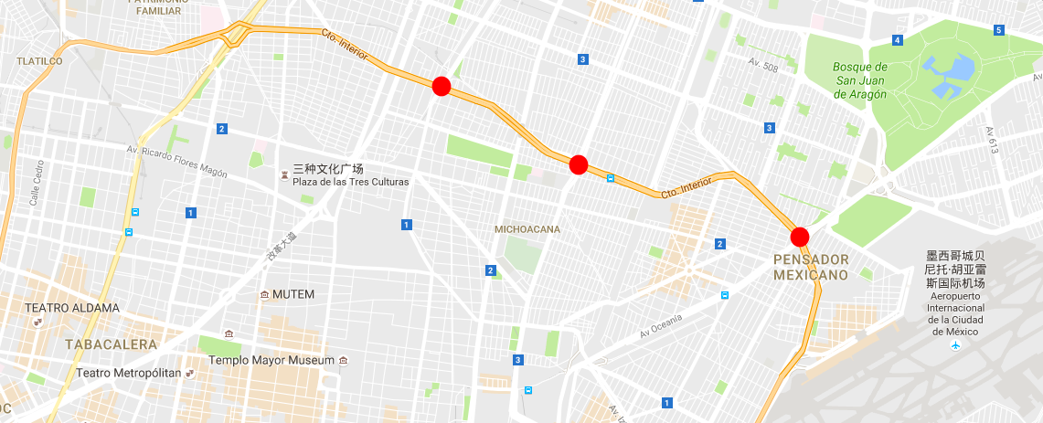
Here is the actual experience: we were in a taxi going to airport via Cto. Interior. We encountered a heavy rain, and several lower points were flooded (indicated as red circles in the following pic).
During the trip, Google Maps kept refreshing the estimated travel time, and the estimated delay for going through those bottlenecks were always increasing. When we arrived, we cost nearly one more hour than the initial estimated travel time.
So how can Google Maps be such inaccurate? And if provided with the information that the capacity in these points will be low for several hours, can we have better estimates?
A queuing model without knowledge in queues
It is almost straightforward to think about a queuing model. To simplify, we consider a serial connection of M/M/1 units and free flow road segments (which can also be seen as M/M/1 unit with $\mu\to\infty$). Following is a visualization of M/M/1 unit (By Tsaitgaist - Mm1.png, CC BY-SA 3.0).

With elementary understanding of queuing theory, I only considered stable case ($\lambda < \ mu$) at first and got into trouble. When the process become stationary, it is impossible to have increasing travel time! In this case, we are actually more likely in an unstable situation: if the capacity remains low forever, the length of the queue will surely explode.
So we just make our first assumption: $\lambda > \mu$. Now, when the difference between $\lambda$ and $\mu$ is not trivial, even with Poisson process as input, we can well assume them as deterministic (constant), since it is unlikely the queue will be empty and we can avoid the nasty analysis in stable case. Or we can argue like this: as $T\to\infty$, total arrival $\sim Poi(\lambda T)$ and total serviced $\sim Poi(\mu T)$, so when $T$ is large enough, the probability to have total serviced amount greater than total arrival is extremely low.
Now we introduce another parameter $\theta$ to describe enter and exit ratios for each road segments between two flooded points. This is quite realistic since people can leave or enter the expressway through ramps. Also, without some inflows we will never have enough arrival to block the next M/M/1 units!
So what is the arrival rate for the middle M/M/1 units? We have $(1-\theta)\mu$ from last unit, and $\theta\lambda$ new inflows. The arrival rate is just the sum of the two. We can also calculate a delay rate $\rho$, which represent how fast delay increases:
$$\rho = \frac{\theta(\lambda - \mu)}{\mu}$$
Now we can summarize our model: we have $n$ M/M/1 units (with same $\lambda$ and $\mu$) with $n-1$ road segments (with same $\theta$ and travel time $T_t$) connecting them in a serial way. We further assume that as we enter this system, every unit already has delay time $T_d$. We further use $T_T$ to denote the sum of $T_t$ and $T_d$.
Calculations
Now it is time to do some high school arithmetics.
Step 0. Upon arrived at the first M/M/1 unit, we are at time $T_1 = 0$, and the queue delay time is $D_1 = T_d$.
Step 1. When arrived at the second M/M/1 unit, we are at time $T_2 = T_1 + D_1 + T_t = T_T$, and the queue delay time at his unit is $D_2 = T_d + \rho T_2 = T_d + \rho T_T = (1+\rho)T_T - T_t$.
Step 2. When arrived at the third M/M/1 unit, we are at time $T_3 = T_2 + D_2 + T_t = (2+\rho)T_T$, and the queue delay time at his unit is $D_3 = T_d + \rho T_3 = (1+\rho)^2 T_T - T_t$.
…
So with induction, it is easy to find total travel time is $T = \frac{(1+\rho)^n-1}{\rho}T_T - T_t$. And the naive initial estimated travel time is $T’ = nT_T - T_t$.
Now let’s replace them with some actual values. First we estimate those parameters:
$$\lambda = 3\text{ lanes}\times 60\text{ km/h} \times 20\text{ veh/km} = 60\text{ veh/min}$$
$$\mu = 1\text{ lanes}\times 4\text{ km/h} \times 300\text{ veh/km} = 20\text{ veh/min}$$
$$\theta = 0.5$$
So
$$\rho = \frac{0.5\times 40}{20} = 1$$
Let $n = 3$ (as in the Mexico City map), we then have $T = 7T_T - T_t$, while $T’ = 3T_T - T_t$; delay is more than 4/3 of the initial estimated travel time! And this is quite similar to what we experienced that afternoon.
Conclusion
So what can we learn from this case study? First, never trust Google Maps in similar situation (which you might only encounter in Mexico City…) and do not take expressway.
Second, stationary results of queuing theory has its limits for application. As we can see, these results are not really useful for this problem, since we are focusing on short term dynamics. We can also explain why so many people find the famous nonlinear time-utilization plot counterintuitive: as utilization $\lambda/\mu\to 1$, the time required to get to the stationary status increase nonlinearly, and in short term dynamics (which is what most people can visualize in their minds) such relationship does not hold! For those who are interested in the asymptotic behavior of the system when $\lambda/\mu\to 1$, you might find the key word heavy traffic approximation useful.
So when should we apply those stationary results? The answer is in planning process, when the arrival variance is large and expected service time is almost infinity. In other cases, simulation is always the safest way to start.