随机性在我们的日常生活中随处可见:股票价格的涨跌,天气的变化以及交通拥堵的产生等现象都与其有关。随机过程理论则提供了一系列简洁有力的工具,不仅能够对这些现象进行建模解释,还为大量工程领域的奠定了分析基础,例如排队系统、最优控制、衍生品定价等。
Stochasticity is pervasive in our daily lives and is related to phenomena like the rise and fall of stock prices, the changes in weather, and the occurrence of traffic congestion. The theory of stochastic processes provides a series of elegant and powerful tools that not only can model these phenomena, but also lay the analytical foundation for a large number of fields and applications, including queueing systems, optimal control problems, and derivative pricing.
在本文和接下来的几篇文章中,我将简要介绍一些随机过程理论中的基本概念及其应用。我主要有两个目标:一是对最近对Durrett的Probability: Theory and Examples一书的学习进行总结,便于未来参考;二则是想要分享和讨论我个人对这些工具的理解与看法。
In this and the next few posts, I will briefly introduce some of the basic concepts in the theory of stochastic processes and their applications. I have two objectives: first, I would like to summarize the recent study of Durrett’s Probability: Theory and Examples for future reference; secondly, I want to share and discuss my understanding and views on these tools.
在开始的几篇文章中,为简便起见,我将主要关注离散时间的随机过程;当我们讨论到布朗运动时我们再开始专注于连续时间随机过程。为了保持符号的一致性,在下面的介绍中我将用$n$表示离散时间过程中的时间,而用$t$表示连续时间过程中的时间。
In the first several posts, for the sake of simplicity, I will mainly focus on the discrete-time processes. We will consider continuous-time processes when we later come to the Brownian motions. For notational consistency, in the following exposition, I will use $n$ for times in discrete-time processes and $t$ for times in continuous-time processes.
随机过程的定义 Definition of Stochastic Processes
首先,让我们回顾一下随机变量的定义。假设有一个由(可能不可观测)的结果$\omega$组成的空间$\Omega$,且在该空间上定义了一个事件集合$\mathcal{F}$和一个概率测度$P$。例如,投掷一枚公平硬币的结果可以描述为
First, let us recall the definition of random variables. Suppose there is a space $\Omega$ consisting of (possibly unobservable) outcomes $\omega$, and this space is equipped with an event set $\mathcal{F}$ and a probability measure $P$. For example, the outcome of a fair coin toss can be described as
$$\omega \in \Omega = \{H,T\}, P(\omega\in \{T\}) = P(\omega\in \{H\}) = 0.5.$$
一个随机变量$X$可以被认为是这些结果在某些可观测空间的投影。换句话说,假设我们的观测值落在空间$S$内,则$X$可以描述为从$\Omega$到$S$的(适应于$\mathcal{F}$的)可测映射。例如,假设Alice与Bob正在对投掷一枚公平硬币的结果进行打赌:如果是正面朝上,Alice能从Bob那里获得一元,反之Alice需要给Bob一元。此时,Alice的收入就是一个关于硬币投掷结果的随机变量$X:\Omega \to \mathbb{R}$,其中$X(H)=1,X(T)=-1$.
A random variable (r.v.) $X$ can be interpreted as a projection of these outcomes onto an observable space. In other words, assuming our observations take places in the space $S$, $X$ can be described as a measurable mapping (adapted to $\mathcal{F}$) from $\Omega$ to $S$. For example, suppose that Alice and Bob are betting on the outcome of a fair coin toss: if it is head, Bob should give Alice $1 and vice versa. Then, Alice’s income is an r.v. $X:\Omega \to \mathbb{R}$ with $X(H)=1,X(T)=-1$.
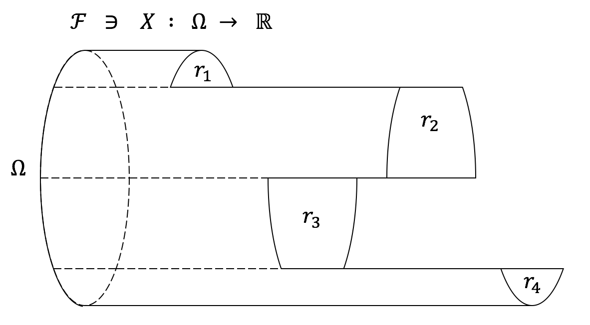
下图是对一般实值随机变量的一种可视化展示:
The following figure is a simple visual illustration of general real-valued r.v.s:
现在,从根据上述定义,我们有两种方式定义一个(实值)随机过程。一方面,如果我们在时间点$\{t_0,\cdots,t_n,\cdots\}$对该过程进行采样,我们可以得到一列随机变量$\{X_{t_i}(\omega_{t_i})\}$以及相应的联合概率测度$\nu_{\{t_0,\cdots,t_n,\cdots\}}$。因此,我们可以将一个随机过程定义为一列对应任意时间$t \in \mathbb{R}^+$的随机变量$\{X_{t}(\omega_{t})\}$,且这些随机变量的任意有限维联合概率测度$\nu_{\{t_0,\cdots,t_n,\cdots\}}$都是一致的。(注:如何正确地定义这里的“一致性”?)
Now, starting from the above definitions, we have two directions to define a (real-valued) stochastic process. On one hand, if we sample the process at time $\{t_0,\cdots,t_n,\cdots\}$, we can obtain a sequence of r.v.s $\{X_{t_i}(\omega_{t_i})\}$ with a specific joint probability measure $\nu_{\{t_0,\cdots,t_n,\cdots\}}$. Following this observation, we can define a stochastic process as a collection of r.v.s $\{X_{t}(\omega_{t})\}$ on time $t \in \mathbb{R}^+$, which is equipped with “consistent” finite-dimensional joint probability measures $\nu_{\{t_0,\cdots,t_n,\cdots\}}$. (Remark: how to formally defined the “consistency” here?)
另一方面,如果我们认为观测值直接就是轨迹或时间序列,那么随机过程可以直接定义为实值序列的随机变量$X(t,\omega)$。换句话说,对于每种可能的结果$\omega$,对应的观测值$X(\cdot,\omega)$是一条实值序列。
On the other hand, if we regard the whole trajectory or time series as the result of a single observation, the stochastic process can be defined directly as an r.v. $X(t,\omega)$ of real-valued sequences. That is, for each possible outcome (or sample) $\omega$, the observation $X(\cdot,\omega)$ is a real-valued sequence.
下面的问题是:这两种定义方式是否一致?幸运的是,Kolmogorov extension theorem给出了正面的回答:对于任意离散时间随机过程和许多连续时间过程(具体来说,那些满足Kolmogorov continuity theorem中的正则性条件的过程),上述两种定义是等价的。
The next question is whether these two directions provide consistent definitions. Luckily, the Kolmogorov extension theorem provides a positive answer: for all discrete-time processes and many continuous-time processes (more specifically, those satisfying the regularity condition in the Kolmogorov continuity theorem), the two definitions are equivalent.
滤子与条件期望 Filtrations and Conditional Expectations
在现实情况下,上面两种随机过程定义方式并不是很有用:确定轨迹上的概率测度或者任意有限维联合概率测度都是不平凡的。由于我们一般对随机过程都有一些历史数据,一种更简便的方式是指定不同时刻观测值的相互依赖性。例如,考虑一个随机游走过程$S_n = X_1 + \cdots + X_n$,其中$X_i$是独立同分布的随机变量。如果我们已知$S_{n-1}=s$,那么$S_n$可以表示为$s + X_n$。
In practice, the two definitions above are not very useful: it is nontrivial to specify either the probability measure on trajectories or the finite-dimensional joint distributions. Because we normally have some historical observations, it is more convenient to specify the process according to the temporal dependency (on the historical observations). For example, consider a random walk $S_n = X_1 + \cdots + X_n$, where $X_i$ are i.i.d. random variables. If we already know $S_{n-1}=s$, we can write $S_n$ as $s + X_n$.
一般来说,对于一个离散时间过程,我们可以按下面的方式根据历史观测值$X_{n-1}, X_{n-2}, \cdots, X_0$指定$X_n$的分布:
In general, for a discrete-time process we can specify the distribution of the observation $X_n$ according to the past observations $X_{n-1}, X_{n-2}, \cdots, X_0$ as follows:
$$X_n \sim P(\cdot|X(n-1,\omega) = x_{n-1}, X(n-2,\omega)=x_{n-2}, \cdots, X(0,\omega)=x_0).$$
不过,当$n$变得很大的时候上面的式子会变得非常冗余。为了简化表达,我们使用$\mathcal{F}_n$代替由历史观测值形成的$\sigma$-代数:$\mathcal{F}_n = \sigma(X_{n}, X_{n-1}, \cdots, X_0)$。换句话说,$\mathcal{F}_n$是一个集合,该集合中的每个元素都是由$\{ X_{n-1}(\omega) \in A_{n-1}, X_{n-2}(\omega)\in A_{n-2}, \cdots, X_{0}(\omega)\in A_0 \}$这种集合经过可数次交并运算生成的。这意味着$\mathcal{F}_n$包含了所有我们关于$X_{n}, X_{n-1}, \cdots, X_0$的信息;然而,由于定义中没有出现具体的观测值$x_{n-1}, x_{n-2}, \cdots, x_0$,$\mathcal{F}_n$应该被理解为从时间0开始向未来看,累积到时间$n$时的所有信息。现在,对任意实际观测序列$x_{n-1}, x_{n-2}, \cdots, x_0$,上述概率分布都可以通过条件概率测度$P(X_n|\mathcal{F}_{n-1})$来表示了。需要注意的是,$P(X_n|\mathcal{F}_{n-1})$这一表达式并不代表任何具体的概率测度,而是一个从信息空间$\mathcal{F}_{n-1}$到概率测度空间的映射。
However, when $n$ becomes large the above representation can be very redundant. To simplify the expression, we denote $\mathcal{F}_n$ as the $\sigma$-algebra generated by the past observations $\mathcal{F}_n = \sigma(X_{n}, X_{n-1}, \cdots, X_0)$. That is, $\mathcal{F}_n$ is a collection of all possible sets generated from $\{ X_{n-1}(\omega) \in A_{n-1}, X_{n-2}(\omega)\in A_{n-2}, \cdots, X_{0}(\omega)\in A_0 \}$. This means that $\mathcal{F}_n$ contains all information we know about $X_{n}, X_{n-1}, \cdots, X_0$; however, because the actual observed values $x_{n-1}, x_{n-2}, \cdots, x_0$ are not specified, $\mathcal{F}_n$ should be interpreted as the (random) information accumulated up to time $n$ when we look into the future from time $0$. Now, for every possible observation sequence $x_{n-1}, x_{n-2}, \cdots, x_0$, the above probability distribution is summarized by the conditional probability measure $P(X_n|\mathcal{F}_{n-1})$. One should notice that $P(X_n|\mathcal{F}_{n-1})$ does not refer to any specific probability measure; in fact, it is a mapping from the information space $\mathcal{F}_{n-1}$ to the probability measure space.
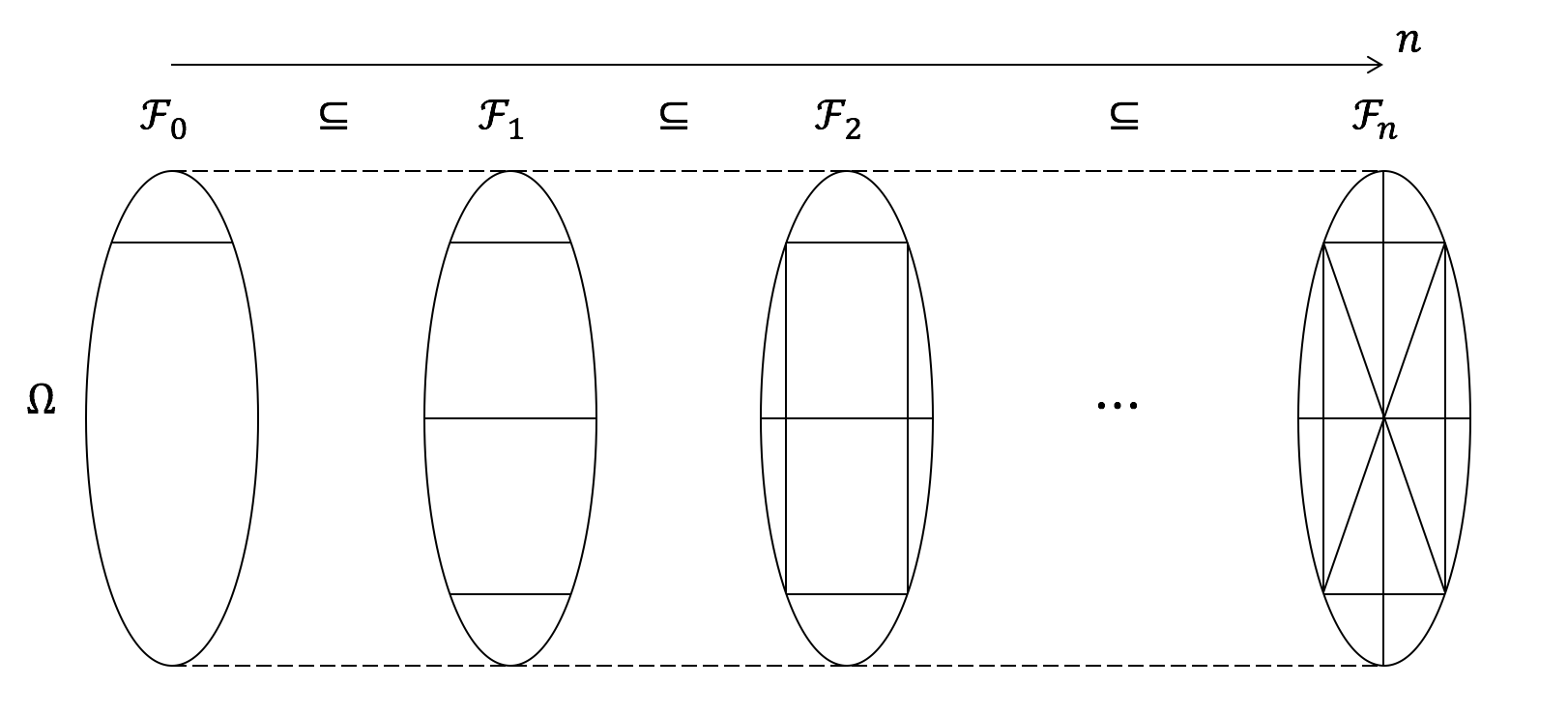
在继续关于条件概率测度的讨论之前,我打算暂时停下,讨论不同$\mathcal{F}_n$之间的关系。由于这些集合表示了随时间累积的“信息”,根据定义,我们应该有一些诸如$\mathcal{F}_0 \subseteq \mathcal{F}_1 \subseteq \cdots \subseteq \mathcal{F}_n$的包含关系。事实上,我们的确可以证明这一点:对任意时间$n_1$时可确定的事件$A\in \mathcal{F}_{n_1}$以及一个未来时间$n_2 > n_1$,$A$也应该在未来可以被确定:$A\in \mathcal{F}_{n_2}$;换句话说,随着时间的推移,旧的信息会被保留,而且新的信息会累积,因此样本空间$\Omega$会被信息集合$\mathcal{F}_n$分割地越来越细。下图形象化地表示了上面这一论断。根据此图,我们也可以清晰地理解为什么数学家们选用了“滤子”这个词来表示信息序列$\{\mathcal{F}_0,\mathcal{F}_1,\cdots\}$。
Before I proceed to discuss the conditional probability measure, I would like to take a break and discuss the relationship among $\mathcal{F}_n$. Because they represent “information” accumulated by time, by definition we should have some inclusion relationships such as $\mathcal{F}_0 \subseteq \mathcal{F}_1 \subseteq \cdots \subseteq \mathcal{F}_n$. And this is in fact what we have: for each event $A$ realized at time $n_1$, that is, $A\in \mathcal{F}_{n_1}$, and a future time $n_2 > n_1$, $A$ should also be realized at time $n_2$: $A\in \mathcal{F}_{n_2}$. In other words, as time goes, the previous knowledge persists and is further complemented with some new knowledge, and the outcome space $\Omega$ can be partition by the information $\mathcal{F}_n$ at finer scales. The following figure should provide a clear illustration of the above comments. And it should also be clear from this figure why mathematicians came up with the word “filtration” for the information sequence $\{\mathcal{F}_0,\mathcal{F}_1,\cdots\}$.
现在,让我们回到条件概率测度$P(X_n|\mathcal{F}_{n-1})$的讨论上来。$\mathcal{F}_{n-1}$的引入虽然简化了表达形式,但是从实际相关关系上没有造成任何差异。因此,除了一些特殊的情况(例如Markov链)外,随着$n$的增长,$P(X_n|\mathcal{F}_{n-1})$会变得非常复杂,难以准确描述。因此,一个自然的问题是,如果我们对于$P(X_n|\mathcal{F}_{n-1})$只有一些简单的信息,我们能否得到任何有意义的结论?事实证明,仅需要期望值信息,我们就能够给出该随机过程的一些重要结构性细节!下面,我将对“期望值信息”这一概念给出明确的定义。
Now let us return to the conditional probability measure $P(X_n|\mathcal{F}_{n-1})$. The introduction of $\mathcal{F}_{n-1}$ simplifies only the notation but not the actual relationship; therefore, except for some special cases such as Markov chains, $P(X_n|\mathcal{F}_{n-1})$ will become very complicated as $n$ grows and may not be accurately specified. Then, a natural question is, can we derive anything useful if we only have some moderate knowledge of $P(X_n|\mathcal{F}_{n-1})$? And it turns out that knowing the expected values alone is enough to provide many important structural details of the process! Next, I will give a clear definition of this concept.
让我们回顾一下:$P(X_n|\mathcal{F}_{n-1})$是一个从信息空间$\mathcal{F}_{n-1}$到概率测度空间的映射。因此,对其直接取期望值会得到一个从$\mathcal{F}_{n-1}$到实值空间的映射。由于$\mathcal{F}_{n-1}$是定义在样本空间$\Omega$上的$\sigma$-代数,为简化表达式,我们希望这个期望值函数能够与某些$\Omega$上的随机变量产生联系。不过,最朴素的做法——将$\mathcal{F}_{n-1}$上的取值直接复制到$\Omega$上——是不可行的,因为同一个样本$\omega$可能会对应多个事件$A \in \mathcal{F}_{n-1}$。然而,如果我们只考虑$\mathcal{F}_{n-1}$中最细粒度的事件,那么这种复制方法是可行的。
Recall that $P(X_n|\mathcal{F}_{n-1})$ is a mapping from the information space $\mathcal{F}_{n-1}$ to the probability measure space; directly taking expectation with respect to $P(X_n|\mathcal{F}_{n-1})$ gives us a mapping from $\mathcal{F}_{n-1}$ to the real space $\mathbb{R}$. Since $\mathcal{F}_{n-1}$ is a $\sigma$-algebra with respect to the outcome space $\Omega$, to simplify the expression, we hope that this expectation can be related to some random variables on $\Omega$. However, the most trivial method, to assign values from $\mathcal{F}_{n-1}$ directly to $\Omega$, is infeasible because the same sample $\omega$ may correspond to several $A$ in $\mathcal{F}_{n-1}$. Nevertheless, it is feasible to do so if we consider the finest partition in $\mathcal{F}_{n-1}$.
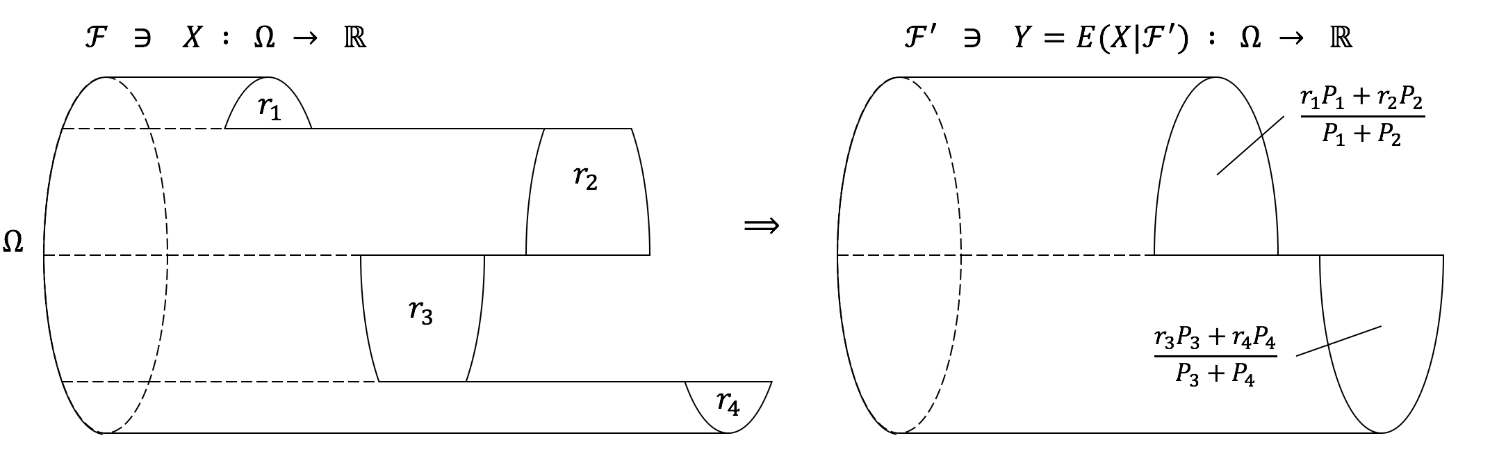
严谨地说,随机变量$Y = E(X|\mathcal{F})$被称为随机变量$X$关于信息$\mathcal{F}$的条件期望,如果它满足以下两个条件:
Formally, random variable $Y = E(X|\mathcal{F})$ is called the conditional expectation of random variable $X$ with respect to information $\mathcal{F}$, if it satisfies the following two conditions:
$$(1) \ Y \in \mathcal{F}; \ (2) \ \forall A \in \mathcal{F}, \int_A Y dP = \int_A X dP.$$
换句话说,第一个条件指出,作为在给定信息$\mathcal{F}$的情况下$X$的估计,$Y$的(切分样本空间$\Omega$的)粒度不能比$\mathcal{F}$更细;第二个条件则指出,对于任意$\mathcal{F}$中发生的事件$A$,$Y$都给出$X$的一个无偏估计。下图是对这两个条件的简单诠释:
In words, the first condition says that $Y$, which is our knowledge of $X$ given information $\mathcal{F}$, cannot be finer than $\mathcal{F}$ (in splitting $\Omega$); while the second condition says that for every possible event in $\mathcal{F}$, $Y$ is an unbiased estimate of $X$. These conditions should be clearly understood by looking at the following figure:
明显,在给定$Y$时,函数$\int_A Y dP: \mathcal{F} \to \mathbb{R}$与上面考虑的对条件概率测度取期望的结果是一致的,因此,上述$Y=E(X|\mathcal{F})$的定义已经足够满足我们的“描述期望值信息”目标了。不仅如此,在某种程度上说,这种定义相比条件概率测度$P(X|\mathcal{F})$的定义对$\mathcal{F}$的本质给出了更简洁准确的表述。
It is clear that given $Y$, the function $\int_A Y dP: \mathcal{F} \to \mathbb{R}$ is consistent with the direct expectation discussed above; so the definition of $Y$ is sufficient for our purpose. Moreover, to some extent, the definition of $E(X|\mathcal{F})$ is more elegant and accurate than the one of conditional probability measure $P(X|\mathcal{F})$ in describing the nature of $\mathcal{F}$.
虽然上述定义很优美,但在实际计算中它相比初等条件概率的定义更难使用(特别对于初学者)。这里,我将通过一个简单的例子来介绍人们一般在计算中会使用到的技巧。考虑条件概率$P(B|A)$,它代表了在事件$A$发生的情况下事件$B$发生的概率;换句话说,$P(B|A)$是条件期望$E(1_B|1_A)$在任一$A$中样本$\omega \in A$上的取值。根据定义,
Though elegant, the above definition is much harder to use for actual computation than the elementary definition of conditional probability, especially for beginners. Here, I will use a simple example to illustrate the techniques people normally used. Consider the conditional probability $P(B|A)$, which represents the probability of occurrence of event $B$ given the occurrence of event $A$; in other words, $P(B|A)$ is the value of conditional expectation $E(1_B|1_A)$ at any $\omega \in A$. By definition,
$$P(B|A)P(A) = \int_A E(1_B|1_A) dP = \int_A 1_B dP = P(A\cap B);$$
因此,我们有
therefore we have
$$P(B|A) = \frac{P(A\cap B)}{P(A)},$$
而这正是条件概率的初等定义。
which is the elementary definition of conditional probability.
停时 Stopping Times
另外一个非常重要的概念是停时。一个(离散时间过程上的)停时是一个定义在$\mathbb{N} \cup \{+\infty\}$上的随机变量,且对应“停”在某些事件发生的时刻。例如,我们可以考虑停时$T=\inf\{n|X_n = H, n \geq 0\}$,它代表着在连续投掷一枚公平硬币的过程中首次出现正面的时间。严谨地来说,一个(离散时间的)适应于滤子$\{\mathcal{F}_n\}$的停时$T$是满足以下条件的一个随机变量:$T: \Omega \to \mathbb{N} \cup \{+\infty \}$,且对于任意$n \in \mathbb{N}$,我们有$\{ T = n\} \in \mathcal{F}_n$。这就是说,选择在时刻$n$停下这一决策是根据时刻$n$已获得的信息$\mathcal{F}_n$作出的,而且不能含有超出$\mathcal{F}_n$范围的信息。
Another very important concept is the stopping time. Intuitively, a stopping time (on discrete-time processes) is a random time, i.e., r.v. on $\mathbb{N} \cup \{+\infty\}$, that “stops” at the (first) occurrence of certain events. For example, we can consider the stopping time $T$ that is the first time to get a head during sequential tosses of a fair coin $T=\inf\{n|X_n = H, n \geq 0\}$. Formally, a (discrete-time) stopping time $T$ adapted to the filtration $\{\mathcal{F}_n\}$ is an r.v. $T: \Omega \to \mathbb{N} \cup \{+\infty \}$ that for every $n \in \mathbb{N}$ we have $\{ T = n\} \in \mathcal{F}_n$. That is, the decision to stop at time $n$ is made with respect to information $\mathcal{F}_n$ accumulated up to time $n$ and cannot contain more information than $\mathcal{F}_n$.
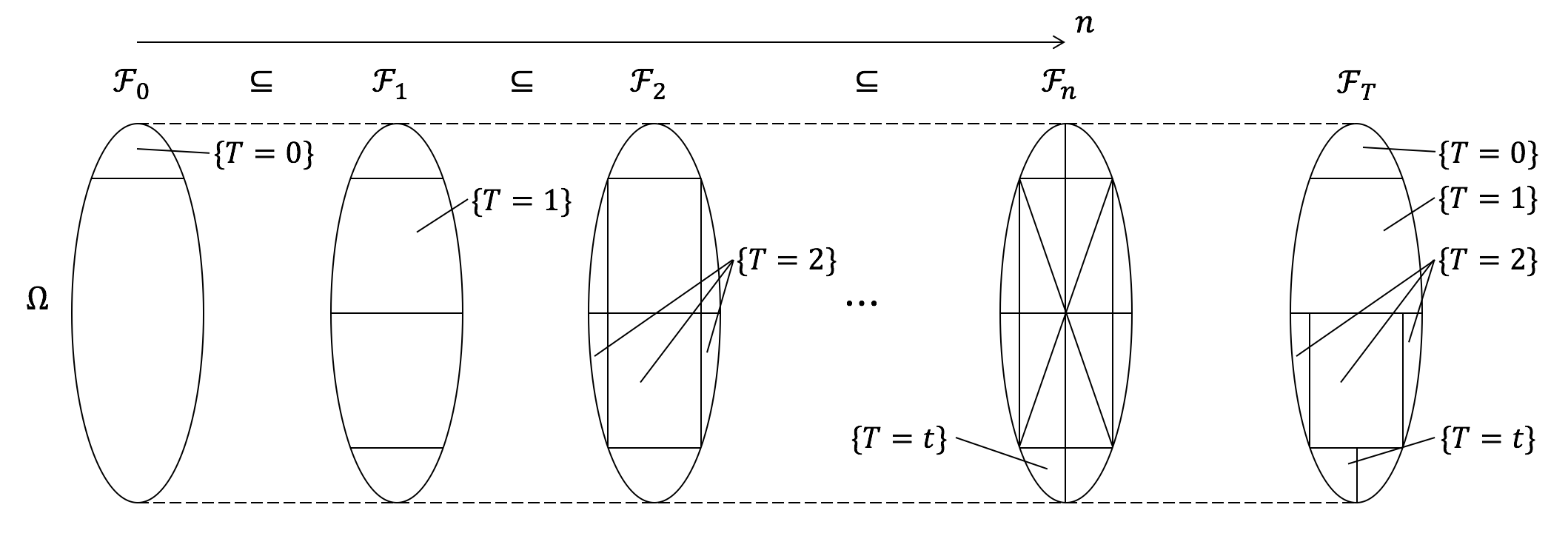
现在,一个自然的问题是如何确定我们在时刻$T$时拥有的信息$\mathcal{F}_T$。明显,如果我们停在了时刻$n$,那么此时我们拥有的信息应该是$\sigma$-代数$\mathcal{F}_{n,T}=\{A\cap \{T=n\}|A\in \mathcal{F}_n\}$。由于事件$\{T=n\}$形成了样本空间$\Omega$的一个划分,信息$\mathcal{F}_T$可以表示为各个划分内子集的并$\{\bigcup A_n|A_n\in \mathcal{F}_n, \ \forall n \in \mathbb{N}\cup \{+\infty\} \}$。然而,一个等价但更简洁的定义是令$\mathcal{F}_T$为$\{A\in \mathcal{F}_{\infty}|A \cap \{ T = n\} \in \mathcal{F}_n, \forall n \in \mathbb{N}\}$。下图简单地展示了上述两种定义方式:
Now, a natural question is to specify the information we have at time $T$, $\mathcal{F}_T$. Obviously, if we stop at time $n$, the information we have is the $\sigma$-algebra $\mathcal{F}_{n,T}=\{A\cap \{T=n\}|A\in \mathcal{F}_n\}$. Since events $\{T=n\}$ form a partition of $\Omega$, $\mathcal{F}_T$ can be expressed as $\{\bigcup A_n|A_n\in \mathcal{F}_n, \ \forall n \in \mathbb{N}\cup \{+\infty\} \}$. An equivalent, but more elegant way is to define $\mathcal{F}_T$ as $\{A\in \mathcal{F}_{\infty}|A \cap \{ T = n\} \in \mathcal{F}_n, \forall n \in \mathbb{N}\}$. The following figure should provide a clear illustration of these two definitions:
停时的主要应用在于将可能发生在不同时间点、但具有非常相似属性的事件聚集在一起,从而简化分析。换句话说,停时可以让我们按观测值$X$对随机过程$X(t,\omega)$进行切片,而不是简单地按样本$\omega$或时间$t$进行切片。这种想法与Lebesgue积分中的想法非常类似:在Lebesgue积分中,求和的对象是具有相似$y$值的微元,而传统的Riemann积分中的求和对象则是具有相似$x$值的微元。下面,我们通过考虑一个经典的计算随机游走过程达到某些具体目标的概率的例子来进一步说明这种思路。考虑一个简单随机游走过程$S_n = X_1 + \cdots + X_n$,其中$X_i$是独立同分布的二项随机变量:$P(-1)=P(1)=0.5$。由Wald等式,对任意满足$ET < \infty$的停时$T$,有
The major applications of stopping time are to align events that are closely related but possibly from different time periods, and simplify analyses. In other words, stopping times allow us to decompose the stochastic process $X(t,\omega)$ according to the observation $X$, rather than the sample $\omega$ or time $t$. This idea is very similar to the intuition behind the Lebesgue integral, which contrasts Riemann integral by taking infinite sums of meshes partitioned according to the range space $\{y\}$. To further illustrate this idea, we consider a classic example that analyzes the probabilities of a random walk to hit some targets. Consider a simple random walk $S_n = X_1 + \cdots + X_n$, where $X_i$ are i.i.d. binomial random variables: $P(-1)=P(1)=0.5$. By Wald’s equation, for any stopping time $T$ with $ET < \infty$ we have
$$ES_T = ET EX_1 = 0.$$
因此,对于任意的$a > 0 > b, a,b \in \mathbb{N}$,如果我们令$T_a$为随机游走首次达到$a$的时间,$T_b$为首次达到$b$的时间,且$T = \min(T_a,T_b)$,那么我们有
Therefore, for any $a > 0 > b, a,b \in \mathbb{N}$, if we let $T_a$ be the first hitting time of $a$ and $T_b$ be the one of $b$, and let $T = \min(T_a,T_b)$, then we have
$$0 = ES_T = aP(T_a < T_b) + bP(T_b < T_a),$$
从而
so
$$P(T_a < T_b) = -\frac{b}{a-b}.$$
注:要应用Wald等式,我们需要说明$ET < \infty$。如何做到这一点?
Remark: to apply Wald’s equation, we need to show $ET < \infty$. How?