在上一篇文章中,我介绍了如何根据关于条件期望的结构性信息(具体来说,条件期望的单调性)来推导一些理论性质和计算一些随机变量的期望值。在这一篇文章中,我将更进一步,讨论如何利用关于条件概率测度$P$的结构性信息。具体来说,我将关注具有以下形式的$P$
In the previous post, I discussed how to use structural information about conditional expectations (specifically, monotonicities of conditional expectations) to derive several theoretical properties and calculate the expected values of some random variables. In this post, I will discuss how to use structural information about the conditional probability measure $P$. Specifically, I will focus on $P$ with the following form
$$P(X_n|\mathcal{F}_{n-1}) = p(X_{n-1},X_n),$$
其中概率转移分布$p$是一个不随时间$n$变化的函数。
in which the transition probability $p$ is a function that is invariant across time $n$.
马尔科夫链的定义 Definition of Markov Chains
首先,我将给出(离散)马尔科夫链的严格定义。假设$(S,\mathcal{S})$是一个可测空间,随机变量$X_n$是从样本空间$\Omega$到$S$上可测映射。若存在函数$p$使得
First, I will give a formal definition of (discrete) Markov chains. Suppose $(S,\mathcal{S})$ is a measurable space, and the random variable $X_n$ is a measurable mapping from the sample space $\Omega$ to $S$. If there exists a function $p$ such that
$$P(X_{n+1}\in A|\mathcal{F}_{n}) = p(X_{n},A), \tag{1.1}$$
那么序列$\{X_n\}$则被认为是一个(相对于$p$的)马尔科夫链。为保证该定义是良定的,函数$p: S\times \mathcal{S} \to R$还需要满足下述条件:
then the sequence $\{X_n\}$ is called a Markov chain (with respect to $p$). To ensure this is well-defined, the function $p: S\times \mathcal{S} \to R$ needs to satisfy the following regular conditions:
对任意$x\in S$,映射$A\to p(x,A)$是空间$(S,\mathcal{S})$上的概率测度;
对任意$A\in \mathcal{S}$,映射$x\to p(x,A)$是一个可测函数。
For any $x\in S$, the mapping $A\to p(x,A)$ is a probability measure on the space $(S,\mathcal{S})$;
For any $A\in \mathcal{S}$, the mapping $x\to p(x,A)$ is a measurable function.
我们称满足以上条件的函数$p$为转移概率。
A function $p$ satisfying the above conditions is said to be a transition probability.
根据上述定义,对每一个马尔科夫链,都存在对应的转移概率函数$p$。下面,我们将进一步说明:若给定一个转移概率函数$p$,我们可以显式地构造任意一个相对于$p$的马尔科夫链。这意味着在讨论马尔科夫链时,我们只需要关注转移概率$p$。
According to the above definition, for each Markov chain, there is a corresponding transition probability $p$. Next, we will show that: if we are given a transition probability $p$, then we can explicitly construct any Markov chain that has $p$ as its transition probability. This means that when discussing the Markov chain, we only need to pay attention to the transition probability $p$.
首先,由于$p$作为条件概率测度确定了历史值$\{X_0,\cdots,X_{n-1}\}$与当前值$X_{n}$的关系,如果进一步给定初始值$X_0$的分布$\mu(B) \equiv P(X_0\in B)$,那么从直觉上我们可以确定序列$\{X_n\}$应具有的任意有限维概率分布。例如,事件$\{X_j\in B_j, 0\leq j\leq n\}$的发生概率可计算如下
First, because $p$, as a conditional probability measure, determines the relationship between the historical value $\{X_0, \cdots, X_{n-1}\}$ and the current value $X_{n}$, if we are further provided with the distribution $\mu(B) \equiv P(X_0\in B)$ of the initial value $X_0$, then intuitively we can determine any finite-dimensional probability distribution of the sequence $\{X_n\}$. For example, the probability of occurrence of the event $\{X_j\in B_j, 0\leq j\leq n\}$ can be calculated as follows
$$P(X_j\in B_j, 0\leq j\leq n) = \int_{B_0}\mu(dx_0)\{ \int_{B_1}p(x_0,dx_1) \cdot \{ \cdots \int_{B_n}p(x_{n-1},dx_n) \} \}. \tag{1.2}$$
其次,当状态空间$(S,\mathcal{S})$满足一定的正则性时,我们可以对上述($\mu$和$p$唯一确定的)有限维概率分布(1.2)运用Kolmogorov延拓定理得到序列空间$(\Omega_o,\mathcal{F}) = (S^{ \{0,1,\cdots\} },\mathcal{S}^{ \{0,1,\cdots\} })$上的一个概率测度$P_{\mu}$,且在$P_{\mu}$下服从有限维概率分布(1.2)的随机变量$X_n$可以被看作是坐标映射$X_n(\omega) = \omega_n$。
Second, when the state space $(S,\mathcal{S})$ is nice, we can apply the Kolmogorov extension theorem on the above finite-dimensional probability distributions (1.2) (which is uniquely determined given $\mu$ and $p$) to obtain a probability measure $P_{\mu}$ on the sequence space $(\Omega_o,\mathcal{F}) = (S^{ \{0,1,\cdots\} },\mathcal{S}^{ \{0,1,\cdots\} })$. Under $P_{\mu}$, the random variable $X_n$ can be viewed as a coordinate map $X_n(\omega) = \omega_n$.
最后,我们可以(通过测度论中的$\pi$-$\lambda$定理和单调类定理)证明:
Finally, we can prove that (by applying the $\pi$-$\lambda$ theorem and the monotone class theorem in the measure theory):
定理1.1:根据上述方式得到的对应概率测度$P_{\mu}$的序列$\{X_n\}$是一个以$p$为转移概率的马尔科夫链。
Theorem 1.1: The coordinate maps $\{X_n\}$ with respect to the probability measure $P_{\mu}$ is a Markov chain with transition probability $p$.
定理1.2:一个以$\mu$为初始分布、$p$为转移概率的马尔科夫链$\{X_n\}$的有限维概率分布服从式(1.2)的形式。
Theorem 1.2: If a Markov chain $\{X_n\}$ has transition probability $p$ and initial distribution $\mu$, then its finite-dimensional probability distributions are given by equation (1.2).
马尔科夫性质 Markov Properties
通过上一节的讨论,我们已经对马尔科夫链的结构有了初步的了解。在这一节中,我将进一步讨论马尔科夫条件(1.1)。具体来说,我将对式(1.1)中隐含的无记忆性这一性质进行更严谨地表述,并将其延拓到更一般的场景中。为此,我们需要(基于上述序列空间$(\Omega_o,\mathcal{F})$的定义)引入平移算子$\theta_n$:
Through the discussion in the previous section, we should have a basic understanding of Markov chains. In this section, I will further discuss the Markov condition (1.1). In particular, I will provide a rigorous description of the memoryless nature implied in equation (1.1) and extend it to more general scenarios. To do so, we need to introduce the shift operator $\theta_n$ (with respect to the definition of the sequence space $(\Omega_o,\mathcal{F})$):
$$\theta_n(\omega) = (\omega_{n},\omega_{n+1},\cdots).$$
基本定理 Fundamental Theorems
首先,我们可以将条件(1.1)从简单事件$\{X_{n+1}\in B\}$推广到更一般的关于未来的有界函数$h(X_{n+1},X_{n+2},\cdots)$上:
First, we can generalize the condition (1.1) from the simple event $\{X_{n+1}\in B\}$ to the more general bounded function $h(X_{n+1}, X_{n+2}, \cdots)$ about the future:
定理2.1(马尔科夫性):假设$Y: \Omega_o \to \mathbb{R}$是一个可测有界函数,则有
Theorem 2.1 (Markov property): Suppose $Y: \Omega_o \to \mathbb{R}$ is a bounded measurable function. Then we have
$$E_{\mu} (Y\circ \theta_m|\mathcal{F}_m) = E_{X_m}Y. \tag{2.1.1}$$
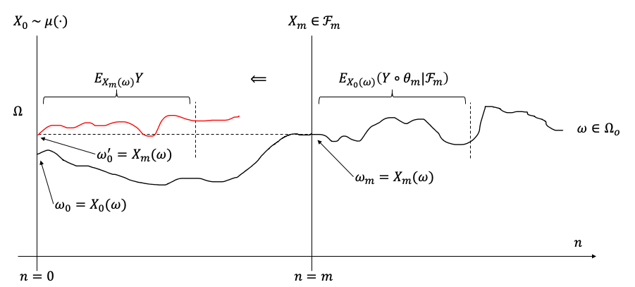
这里,我尝试通过下图对定理2.1的含义给出一个直观的诠释。下图展示了一条序列空间$\Omega_o$中的样本轨迹$\omega$,其中右上角关于真实样本$\omega$(黑色线)的括号部分对应式(2.1.1)的左端,而左上角关于虚拟样本$\omega’$(红色线)的括号部分对应式(2.1.1)的右端。马尔科夫性质(定理2.1)说明,红黑两线在括号截取的部分应在统计意义上完全一致(注:但从单个样本轨迹的角度来看不一定一致,如下图所示)。这意味着轨迹$\omega$在时间$n < m$的部分对$n > m$的部分没有影响,即马尔科夫链是不具有记忆性的。
Here, I will try to give an intuitive interpretation of theorem 2.1 with the following figure. The following figure shows a sample trajectory $\omega$ (the black line) in the sequence space $\Omega_o$, where the bracket in the upper right corner on the real sample $\omega$ (the black line) corresponds to the left-hand side of the equation (2.1.1), and the brackets on the artificial sample $\omega’$ (the red line) in the upper left corner corresponds to the right-hand side of the equation (2.1.1). The Markov property (theorem 2.1) shows that the parts within the brackets from the red and black lines should be statistically identical (Note: But the two sample trajectories are not necessarily identical, as shown in the following figure). This means that the part of the trajectory $\omega$ at time $n < m$ does not affect the part of $n > m$, i.e., the Markov chain is memoryless.
下面,我简单介绍一下该定理的证明思路。证明的主要目标是说明下式对任意满足条件的$Y$和$A\in \mathcal{F}_m$成立:
Next, I will introduce the basic ideas behind the proof of the theorem. The main target is to show for any regular $Y$ and $A\in \mathcal{F}_m$ that the following equation holds:
$$E_{\mu} (Y\circ \theta_m \cdot 1_{A}) = E_{\mu} (E_{X_m}Y \cdot 1_{A}). \tag{2.1.2}$$
具体通过以下三步完成证明:1)基于概率测度$P_{\mu}$的形式(1.2),证明式(2.1.2)对具有形式$\prod_{m=0}^n g_m(X_m)$的$Y$以及具有形式$\{X_0\in A_0,\cdots,X_n \in A_n\}$的$A$成立;2)通过$\pi$-$\lambda$定理将式(2.1.2)延拓到任意$A\in \mathcal{F}_m$;3)通过单调类定理将式(2.1.2)延拓到任意满足条件的$Y$。
The detailed proof can be summarized in three steps: 1) Based on the form of probability measure $P_{\mu}$ (1.2), prove that equation (2.1.2) holds for $Y$ in form $\prod_{m=0}^n g_m(X_m)$ and $A$ in form $\{X_0\in A_0,\cdots,X_n \in A_n\}$. 2) Extend the result in 1) to any $A\in \mathcal{F}_m$ by the $\pi$-$\lambda$ theorem; 3) Extend the result in 2) to any regular $Y$ by the monotonic class theorem.
下面的定理进一步将马尔科夫性推广到含有停时的场景中。
The following theorem further generalizes the Markov property to scenarios with stopping times.
定理2.2(强马尔科夫性):假设对于任意$n \in \mathbb{N}, Y_n: \Omega_o \to \mathbb{R}$是可测有界函数,且一致有界:$|Y_n|\leq M$。则对任意停时$T$,有
Theorem 2.2 (strong Markov property): Suppose for any $n \in \mathbb{N}, Y_n: \Omega_o \to \mathbb{R}$ is a measurable bounded function, and they are uniformly bounded $|Y_n|\leq M$. Then for any stopping time $T$,
$$E_{\mu} (Y_T \circ \theta_T|\mathcal{F}_T) = E_{X_T}Y_T \text{ on } \{T < \infty\}. \tag{2.1.3}$$
证明:根据条件期望的定义,我们只需要证明$\forall A \in \mathcal{F}_T$,有
Proof: According to the definition of conditional expectations, we only need to prove $\forall A \in \mathcal{F}_T$ the following equation holds
$$E_{\mu}(1_{A \cap \{T < \infty \}}\cdot E_{X_T}Y_T) = E_{\mu}(1_{A \cap \{T < \infty \}} \cdot Y_T \circ \theta_T). \tag{2.1.4}$$
而事实上,由于$A \cap \{T = n \} \in \mathcal{F}_n$,因此根据定理2.1,有
However, because $A \cap \{T = n \} \in \mathcal{F}_n$ for each $n$, we can apply theorem 2.1 to obtain
$$E_{\mu} (1_{A \cap \{T = n \} } \cdot Y_n \circ \theta_n) = E_{\mu} (1_{A \cap \{T = n \} } \cdot E_{X_n}Y_n); \tag{2.1.5}$$
对上式中的$n$求和即得式(2.1.4)。Q.E.D.
and summing the equation above leads to the equation (2.1.4). Q.E.D.
例子 Examples
在这一小节中,我将通过两个例子来展示一些使用马尔科夫性质(定理2.1、2.2)的技巧。在下列及后续小节的讨论中,我们往往会考虑确定的起始状态$X_0 = x$;此时我们将对应的(序列空间上的)概率测度$P_{\delta_x}$简记为$P_x$。
In this subsection, I will illustrate through two examples some techniques in applying the Markov properties (theorems 2.1 and 2.2). In the following discussions, we usually will consider a deterministic initial state $X_0 = x$; at that time we will use shorthand notation $P_x$ for the (sequence space) probability measure $P_{\delta_x}$.
例子2.1:根据条件期望的性质和马尔科夫性(定理2.1),可得
Example 2.1: According to the properties of conditional expectation and the Markov property (theorem 2.1), we have
$$\begin{aligned} P_x(X_{m+n} = z) & = E_x(P_x(X_{m+n} = z | F_m)) = E_x(E_x(1_{\{X_{n} = z\}} \circ \theta_m | F_m)) \\ & = E_x(P_{X_m}(X_{n} = z)) = \sum_y P_y(X_n = z)\cdot P_x(X_m = y). \end{aligned} \tag{2.2.1}$$
例子2.2(反射原理):令$x_1,x_2,\cdots$为分布关于0对称的独立同分布随机变量。又令$S_n = \sum_{m=1}^{n} x_m$。若$a>0$,则
Example 2.2 (Reflection Principle): Let $x_1,x_2,\cdots$ be i.i.d. random variables with a distribution symmetric about 0. Let $S_n = \sum_{m=1}^{n} x_m$. If $a>0$, then
$$P(\sup_{m \leq n} S_m > a) \leq 2P(S_n > a). \tag{2.2.2}$$
证明:一方面,考虑停时$T = \inf\{m\leq n: S_m > a\}$;该随机变量表示序列$\{S_n\}$首次突破$a$的时间。容易看出
Proof: On the one hand, let us consider stopping time $T = \inf\{m\leq n: S_m > a\}$, which represents the time the chain $\{S_n\}$ first exceeds $a$. It is obvious that
$$P(\sup_{m \leq n} S_m > a) = P(T < \infty) = E_0 1_{\{T \leq n\}}. \tag{2.2.3}$$
另一方面,考虑随机变量$Y_m = 1_{\{S_{n-m} > a\}}$。容易看出,$Y_m \circ \theta_m = 1_{\{S_{n} > a\}}$对任意$m\leq n$成立。因此
On the other hand, let us consider random variables $Y_m = 1_{\{S_{n-m} > a\}}$. It is obvious that $Y_m \circ \theta_m = 1_{\{S_{n} > a\}}$ holds for any $m\leq n$; therefore,
$$P(S_n > a) = E_0(1_{\{S_{n} > a\}} \cdot 1_{\{T \leq n\}}) = E_0(Y_T \circ \theta_T \cdot 1_{\{T \leq n\}}). \tag{2.2.4}$$
现在,根据强马尔科夫性(定理2.2)可知
Now, according to the strong Markov property (theorem 2.2),
$$E_0(Y_T \circ \theta_T \cdot 1_{\{T \leq n\}}) = E_0(E_0(Y_T \circ \theta_T|\mathcal{F}_T)\cdot 1_{\{T \leq n\}}) = E_0(E_{S_T}Y_T\cdot 1_{\{T \leq n\}}). \tag{2.2.5}$$
最后,注意到在事件$\{T \leq n\}$上有$S_T > a$,因此根据$x_n$的分布对0的对称性,在事件$\{T \leq n, Y_T = y\}$上有
Finally, because $S_T > a$ on event $\{T \leq n\}$, we can derive the following result on event $\{T \leq n, Y_T = y\}$ by leveraging the symmetry of $x_n$’s distribution about 0:
$$E_{S_T}Y_T\ = P_{y}(S_{n-T} > a) \geq P_{y}(S_{n-T} \geq y) = \frac{1}{2}. \tag{2.2.6}$$
综合式(2.2.3)-(2.2.6)即得证。Q.E.D.
The proof is now completed according to equations (2.2.3)-(2.2.6). Q.E.D.
渐近性质 Asymptotic Behavior
常返性与时均收敛性 Recurrence and Time-Average Convergence
在上一节中,我介绍了马尔科夫链的无记忆性本质。这种性质所造成的一个后果是,如果该序列从状态$y$出发几乎一定能够返回$y$,那么该序列在未来一定能够无穷多次返回状态$y$;这种性质被称为常返性。在这一小节中,我将详细介绍该性质及其他一些类似的性质。
In the previous section, I discussed the memoryless nature of Markov chains. This property implies that, if the chain is almost surely able to return to state $y$ starting from $y$, then the chain must return to $y$ infinitely many times in the future. This property is called recurrence. In this section, I will introduce this property and some other similar properties in detail.
让我们记马尔科夫链$\{X_n\}$第$k$次回到状态$y$的时间为$T_y^k = \inf\{n > T_y^{k-1}: X_n = y\}$(假设$T_y^0 = 0$),并将首次回归时间$T_y^1$简记为$T_y$。令$\rho_{xy} = P_x(T_y < \infty)$为事件“从状态$x$出发,最终能够返回/到达状态$y$”的发生概率。下面的定理说明:事件“多次返回状态$y$”可以看成是事件“单次返回状态$y$”的多次重复。
Let us denote the time of the chain $\{X_n\}$’s $k$-th return to state $y$ as $T_y^k = \inf\{n > T_y^{K-1}: X_n = y\}$ (assuming $T_y^0 = 0$), and use the shorthand notation $T_y$ for the first return time $T_y^1$. Let $\rho_{xy} = P_x(T_y < \infty)$ be the probability of the existence of a single return to state $y$ starting from $x$. The following theorem states that the event “multiple returns to $y$” can be viewed as repetitions of the event “(single) return to $y$”.
定理3.1:$P_x(T_y^k < \infty) = \rho_{xy}\rho_{yy}^{k-1}$。
Theorem 3.1: $P_x(T_y^k < \infty) = \rho_{xy}\rho_{yy}^{k-1}$.
证明:令$Y = 1_{\{ T_y < \infty\} }$。一方面,根据强马尔科夫性质(定理2.2),有
Proof: Let $Y = 1_{\{ T_y < \infty\} }$. On the one hand, according to the strong Markov property (theorem 2.2), we have
$$E_{x} (Y \circ \theta_{T_y^k}|\mathcal{F}_{T_y^k}) = E_{X_{T_y^k}}Y = E_yY = \rho_{yy} \text{ on } \{T_y^k < \infty\} \tag{3.1.1}$$
对任意$k \geq 1$成立。另一方面,容易看出
holds for any $k \geq 1$. On the other hand, it is obvious that
$$P_x(T_y^k < \infty) = E_x(1_{\{T_y^k < \infty\}}) = E_x(Y \circ \theta_{T_y^{k-1}} \cdot 1_{\{T_y^{k-1} < \infty\}}) = E_{x}( E_{x} (Y \circ \theta_{T_y^{k-1}} \cdot 1_{\{T_y^{k-1} < \infty\}}|\mathcal{F}_{T_y^{k-1}})). \tag{3.1.2}$$
由于事件$\{T_y^{k-1} < \infty\} \in \mathcal{F}_{T_y^{k-1}}$,因此根据条件期望的性质和以上两式,当$k \geq 2$时,有
Because event $\{T_y^{k-1} < \infty\} \in \mathcal{F}_{T_y^{k-1}}$, according to the properties of conditional expectations and equation (3.1.1)-(3.1.2), the following equation holds when $k \geq 2$
$$P_x(T_y^k < \infty) = E_{x}( E_{x} (Y \circ \theta_{T_y^{k-1}}|\mathcal{F}_{T_y^{k-1}}) \cdot 1_{\{T_y^{k-1} < \infty\}}) = E_{x}(\rho_{yy} \cdot 1_{\{T_y^{k-1} < \infty\}}) = \rho_{yy} P_x(T_y^{k-1} < \infty). \tag{3.1.3}$$
根据上式、$P_x(T_y^1 < \infty) = \rho_{yy}$和归纳法即得证。Q.E.D.
The remaining proof should be obvious given equation (3.1.3) and $P_x(T_y^1 < \infty) = \rho_{yy}$. Q.E.D.
根据定理3.1,我们知道如果$\rho_{yy} = 1$,那么对任意$k\geq 1$,$P_y(T_y^k < \infty) = 1$,即序列$\{X_n\}$以概率1一直返回到状态$y$上。基于此,我们可以将一个状态$y$的常返性定义为$\rho_{yy} = 1$,并相应地将非常返性定义为$\rho_{yy} < 1$。
According to theorem 3.1, we know that if $\rho_{yy} = 1$, then for any $k\geq 1$, $P_y(T_y^k < \infty) = 1$, i.e., the sequence $\{X_n\}$ returns to state $y$ infinitely with probability 1. Based on this, we can define the recurrence of the state $y$ as $\rho_{yy} = 1$, and define the transience as $\rho\ _{yy} < 1$.
下一步,我们考虑到达/返回次数$N_y = \sum_{m=1}^{\infty} 1_{\{X_m = y\}}$。根据定理3.1,
Next, let us consider the number of visits $N_y = \sum_{m=1}^{\infty} 1_{\{X_m = y\}}$. According to theorem 3.1, we have
$$E_xN_y = \sum_{k=1}^{\infty}P_x(N_y \geq k) = \sum_{k=1}^{\infty}P_x(T_y^k < \infty) = \rho_{xy} \sum_{k=1}^{\infty}\rho_{yy}^{k-1} = \frac{\rho_{xy}}{1 - \rho_{yy}}. \tag{3.1.4}$$
因此我们可得以下定理:
Therefore we have the following theorem:
定理3.2:状态$y$是常返的,当且仅当$E_yN_y = \infty$。
Theorem 3.2: State $y$ is recurrent, if and only if $E_yN_y = \infty$.
上述定理说明,对于一个常返的状态$y$,其到达次数的期望是无穷的。下面的定理则进一步分析了到达该状态的频率。
Theorem 3.2 shows that the expected number of visits to a recurrent state $y$ is infinity. The following theorem further analyzes the frequency of visits.
定理3.3:若状态$y$常返,则对任意初始状态$X_0 = x\in S$,
Theorem 3.3: If state $y$ is recurrent, then for any initial state $X_0 = x\in S$,
$$\begin{aligned} & \lim_{n\to\infty} \frac{N_y^n}{n} = \frac{1}{E_yT_y}1_{\{T_y<\infty\}}, \ P_x\text{-a.s.}; \\ & \lim_{n\to\infty} \frac{E_xN_y^n}{n} = \frac{\rho_{xy}}{E_yT_y}, \end{aligned} \tag{3.1.5}$$
其中$N_y^n = \sum_{m=1}^n 1_{\{X_m=y\}}$代表在时间$n$的到达次数。
in which $N_y^n = \sum_{m=1}^n 1_{\{X_m=y\}}$ is the number of visits by time $n$.
证明:容易看出第二式即对第一式求期望;因此我们只需考虑证明第一式。
Proof: It is obvious that the second equation results from taking expectations with respect to the first equation, so we only need to prove the first.
在上面的讨论中,曾引入了变量$T_y^k$以表示第$k$次到达状态$y$的时间。现在,考虑相邻两次到达时间的间隔$t_k = T_y^k - T_y^{k-1}$。若令$t$为$X_0 = y$时的$t_1$,则$t_k = t \circ \theta_{T_y^{k-1}}$对于$k \geq 2$成立。由于$y$常返,因此$P(T_y^{k-1} < \infty) = 1$,从而根据强马尔科夫性质(定理2.2),对任意有界函数$f$有
In discussions above, I have introduced random variable $T_y^k$ for the time of the $k$-th visits to $y$. Let us now consider the interarrival time $t_k = T_y^k - T_y^{k-1}$. If we denote the $t_1$ under $X_0 = y$ as $t$, then $t_k = t \circ \theta_{T_y^{k-1}}$ for any $k \geq 2$. Since $y$ is recurrent, $P(T_y^{k-1} < \infty) = 1$. So according to the strong Markov property (theorem 2.2), for any bounded function $f$ we have
$$E_{x} (f(t_k)|\mathcal{F}_{T_y^{k-1}}) = E_{x} (f(t) \circ \theta_{T_y^{k-1}}|\mathcal{F}_{T_y^{k-1}}) = E_{X_{T_y^k}}f(t) = E_yf(t), \ P_x\text{-a.s.}, \tag{3.1.6}$$
从而$t_k$与$\mathcal{F}_{T_y^{k-1}}$独立。由于变量$t_0,\cdots,t_{k-1}$都在信息集$\mathcal{F}_{T_y^{k-1}}$中,因此$t_k(k\geq 2)$是独立同分布的随机变量。进而根据强大数定律,有
Therefore, $t_k$ is independent from $\mathcal{F}_{T_y^{k-1}}$. Since the random variables $t_0,\cdots,t_{k-1}$ are all in the information $\mathcal{F}_{T_y^{k-1}}$, the $t_k(k\geq 2)$s are i.i.d. random variables. Then, applying the strong law of large numbers on these $t_k$s, we have
$$\frac{T_y^k-T_y}{k} = \frac{\sum_{i=2}^k t_i}{k} \to E_y T_y, \ P_x\text{-a.s.}. \tag{3.1.7}$$
现在,对两类事件分别讨论:
Next, we consider two cases:
1)在事件$\{T_y = \infty\}$中,$N_y^n \equiv 0$,因此
1)On $\{T_y = \infty\}$, $N_y^n \equiv 0$, so
$$\frac{N_y^n}{n} \equiv 0 \text{ on } \{T_y = \infty\}.$$
2)在事件$\{T_y < \infty\}$中,$T_y/k \to 0$,因此由式(3.1.7),有
2)On $\{T_y < \infty\}$, $T_y/k \to 0$, so according to equation (3.1.7), we have
$$\frac{T_y^k}{k} \to E_y T_y, \ P_x\text{-a.s.}. \tag{3.1.8}$$
又根据$T_y^k = \inf\{n\geq 1:N_y^n = k\}$,有$T_y^{N_y^n} \leq n < T_y^{N_y^n+1}$,从而有以下不等式放缩:
Because $T_y^k = \inf\{n\geq 1:N_y^n = k\}$, $T_y^{N_y^n} \leq n < T_y^{N_y^n+1}$, and we can approximate the value of $\frac{n}{N_y^n}$ as follows
$$\frac{T_y^{N_y^n}}{N_y^n} \leq \frac{n}{N_y^n} < \frac{T_y^{N_y^n+1}}{N_y^n+1}\frac{N_y^n+1}{N_y^n}. \tag{3.1.9}$$
再注意到由于$y$的常返性,$N_y^n\to \infty$;因此在上式中取极限$n \to \infty$并引入式(3.1.8)的结果,即得
Since $y$ is recurrent, $N_y^n\to \infty$; so by letting $n \to \infty$ in equation (3.1.9) and incorporating results in equation (3.1.8), we have
$$\frac{n}{N_y^n} \to E_y T_y, \ P_x\text{-a.s.}.$$
现在,综合1)和2)的结果即得证。Q.E.D.
Now the statement is clear given results from both parts 1) and 2). Q.E.D.
乍一看,定理3.3给出的结果是平凡的:序列$\{X_n\}$到达状态$y$的频率是相邻返回时间间隔的期望$E_yT_y$。不过,当$E_yT_y = \infty$时,定理3.2和3.3共同给出了有意思的结果:平均到达$y$的总次数是正无穷,但是平均每时刻到达频率却是0。在这种情况下,状态$y$被称为零常返;与之相对应地,若$E_yT_y<\infty$,则状态$y$被称为正常返。
At first glance, theorem 3.3 is trivial: the frequency of visits to state $y$ is the inverse of the expected interarrival time $E_yT_y$. However, when $E_yT_y = \infty$, theorem 3.2 and 3.3 together give an interesting result: the expected number of visits to $y$ is infinity, but the frequency of visits is zero. In this case, state $y$ is said to be null recurrent; correspondingly, if $E_yT_y<\infty$, the state $y$ is said to be positive recurrent.
遍历性质与空间平均收敛性 Asymptotic Property and Space-Average Convergence
在上一小节中,我介绍了马尔科夫链$\{X_n\}$在单个状态$y$处的渐近性质。在这一小节中,我将介绍该序列在整个状态空间$S$上的渐近性质。限于篇幅,这里我们不妨假设$S$是可列的,以简化讨论的难度。
In the previous subsection, I introduced the asymptotic behavior of the Markov chain $\{X_n\}$ on a specific state $y$. In this subsection, I will introduce the asymptotic behavior of the chain over the entire state space $S$. Due to space limitations, here we assume that $S$ is countable to simplify the subsequent discussion.
我们首先给出一个能够将单个状态处的常返性质推广到其他状态上的充分条件:
First, let me give a sufficient condition for transferring the recurrence property of a specific state to other states:
定理3.4:若状态$x$常返,且$\rho_{xy} > 0$,则状态$y$也是常返的,且$\rho_{yx} = 1$。
Theorem 3.4: If state $x$ is recurrent, and $\rho_{xy} > 0$, then state $y$ is also recurrent, and $\rho_{yx} = 1$.
证明:令$p^k(x,y)$代表从状态$x$出发经过恰好$k$步到达状态$y$的概率。由于$\sum_{k=0}^{\infty}p^k(x,y) \geq \rho_{xy} > 0$,因此$K = \inf\{k:p^k(x,y) > 0\} < \infty$。根据$p^K(x,y) > 0$以及$S$的可列性可知,存在一条路径$x,y_1,\cdots,y_{K-1},y$使得$p(x,y_1)\cdots p(y_{K-1},y)>0$成立。现在,根据
Proof: Let $p^k(x,y)$ be the probability of starting from $x$ and arriving at $y$ in exactly $k$ steps. Since $\sum_{k=0}^{\infty}p^k(x,y) \geq \rho_{xy} > 0$, $K = \inf\{k:p^k(x,y) > 0\} < \infty$. Now, because $S$ is countable, there must exist a path $x,y_1,\cdots,y_{K-1},y$ such that $p(x,y_1)\cdots p(y_{K-1},y)>0$. Now, from
$$0 = 1 - \rho_{xx} = P_x(T_x = \infty) \geq p(x,y_1)\cdots p(y_{K-1},y)(1 - \rho_{yx}), \tag{3.2.1}$$
可得$\rho_{yx} = 1$。
we know that $\rho_{yx} = 1$.
接下来,由于$\rho_{yx} > 0$,重复上面的推导可知$L = \inf\{l:p^l(y,x) > 0\}< \infty$。又基于$x$的常返性和定理3.2,有
Next, because $\rho_{yx} > 0$, we can replicate the derivation above to show $L = \inf\{l:p^l(y,x) > 0\}< \infty$. Then, according to the recurrence of $x$ and theorem 3.2, we have
$$\sum_{n=0}^{\infty}p^{K+L+n}(y,y) \geq \sum_{n=0}^{\infty} p^L(y,x)p^n(x,x)p^K(x,y) = p^L(y,x)p^K(x,y) \sum_{n=0}^{\infty}p^n(x,x) = \infty. \tag{3.2.2}$$
对式(3.2.2)的结果再次应用定理3.2即得$y$的常返性。Q.E.D.
The recurrence of $y$ can then be derived by applying theorem 3.2 on equation (3.2.2). Q.E.D.
定理3.4说明,性质$\rho_{xy} > 0$能够将状态$x$的常返性传递到状态$y$上。我将这种性质定义为(单向的)连通性。进一步地,如果一个集合$D$满足对任意状态对$x,y\in D$都有$\rho_{xy} > 0$$,那么我们将其称为全联通或不可约。根据定理3.4可知,在一个不可约的集合$D$中,如果其中一个状态$x$是常返的,那么$D$中的所有其他状态都是常返的;故我们可以称常返性是一种“类性质”。又因为$\rho_{xy} = 0$意味着从状态$x$出发几乎不可能到达状态$y$,因此如果序列$\{X_n\}$的初始状态$X_0 = x$属于某个不可约集合$D$,那么该序列的后续轨迹都将以概率1完全落在$D$中。这意味着后续对渐近分布的讨论可以不失一般性地假设$S$是不可约的。
Theorem 3.4 shows that $\rho_{xy} > 0$ can transfer the recurrence of state $x$ to state $y$. I define this property as the (directional) connectivity. Moreover, if for any state $x, y$ in a set $D$ $\rho_{xy} > 0$ holds, then we call $D$ fully-connected or irreducible. According to theorem 3.4, if there exists a recurrent state $x$ in the irreducible set $D$, then all other states in $D$ are recurrent; therefore, recurrence can be viewed as a “class property”. Moreover, because $\rho_{xy} = 0$ means that it is almost impossible to reach the state $y$ starting from the state $x$, if the initial state $X_0 = x$ of the sequence $\{X_n\}$ belongs to an irreducible set of $D$, then the subsequent trajectory of the sequence will stay completely in $D$ with probability 1. This means that in the subsequent discussion of asymptotic distributions we can assume without loss of generality that $S$ is irreducible.
下面,我们进一步考虑序列$\{X_n\}$的渐近分布。容易注意到,如果随机变量$X_n$按分布收敛到某个概率测度$\pi$,那么根据转移概率$p$的定义,该分布需要满足条件
Next, we consider the asymptotic distribution of the chain $\{X_n\}$. According to the definition of the transition probability $p$, if $X_n$ converges in distribution to $\pi$, then $\pi$ must satisfy
$$(1) \ \sum_{x\in S} \pi(x) p(x,y) = \pi(y). \tag{3.2.3}$$
然而,满足条件(1)的不一定是一个概率测度;在状态空间$S$的元素是可列的情况下,一个概率分布还需要满足以下正则性条件:
However, (1) is not a sufficient condition for $\pi$ to be a probability measure; to ensure it is one, we need the following condition in cases that $S$ is countable:
$$(2) \ \sum_{x\in S} \pi(x) = 1. \tag{3.2.4}$$
下面,我们将满足条件(1)、但不一定满足条件(2)的测度称为平稳测度,并用$\mu$表示;同时满足条件(1)和(2)的则称为平稳分布,用$\pi$表示。下面的定理给出了一种平稳测度的构造方式。
In the subsequent discussion, we call a measure satisfying condition (1) as stationary measure and denote it as $\mu$, and a measure satisfying both conditions (1) and (2) as stationary probability and denote it as $\pi$. The next theorem provides a method to construct stationary measures.
定理3.5:若状态$x$常返,则
Theorem 3.5: If state $x$ is recurrent, then
$$\mu_x(y) = E_x(1_{\{X_0 = y\}} + N_y^{T_x-1}) = \sum_{n=0}^{\infty} P_x(X_n=y,T_x>n) \tag{3.2.5}$$
定义了一个平稳测度。
defines a stationary measure.
证明:根据定义式(3.2.5)并应用Fubini定理交换和式,我们可以得到
Proof: Applying Fubini Theorem and equation (3.2.5), we have
$$\sum_{y \in S} \mu_x(y) p(y,z) = \sum_{n=0}^{\infty} \sum_{y \in S} p(y,z) P_x(X_n=y,T_x>n). \tag{3.2.6}$$
当$z \neq x$时,有
On the one hand, when $z \neq x$,
$$\sum_{y \in S} p(y,z) P_x(X_n=y,T_x>n) = \sum_{y \in S} P_x(X_n=y,X_{n+1}=z,T_x>n+1) = P_x(X_{n+1}=z,T_x>n+1);$$
将上式回代到式(3.2.6)中,并应用式(3.2.5)的定义,即得
substituting the above result into equation (3.2.6), we have
$$\sum_{y \in S} \mu_x(y) p(y,z) = \sum_{n=0}^{\infty}P_x(X_{n+1}=z,T_x>n+1) = \mu_x(z). \tag{3.2.7}$$
而当$z = x$时,有
On the other hand, when $z = x$,
$$\sum_{y \in S}p(y,z) P_x(X_n=y,T_x>n) = \sum_{y \in S}P_x(X_n=y,X_{n+1}=x,T_x=n+1) = P_x(T_x=n+1);$$
因此有
Therefore, we have
$$\sum_{y \in S} \mu_x(y) p(y,z) = \sum_{n=0}^{\infty}P_x(T_x=n+1) = 1 = \mu_x(x). \tag{3.2.8}$$
综合式(3.2.7)及(3.2.8)即得证。Q.E.D.
The proof is now completed according to equations (3.2.7) and (3.2.8). Q.E.D.
定理3.5说明了若存在某个状态常返,那么平稳测度$\mu$存在。反过来,我们可以证明:若状态空间$S$不可约,且存在某个状态常返,那么平稳测度在考虑数乘变换下是唯一的;即对两个平稳测度$\mu_1,\mu_2 \neq 0$,必存在一个实数$c$使得$\mu_2 = c\mu_1$。碍于篇幅,这里将不展开讨论该结论,感兴趣的读者可以在Durrett的概率论教材的第6.5节找到相关内容。
Theorem 3.5 shows the existence of stationary measures $\pi$ when there is a recurrent state. Conversely, we can prove that if the state space $S$ is irreducible and there is a recurrent state, then the stationary measure $\pi$ is unique up to constant multiples, i.e., for two stationary measures $\mu_1,\mu_2 \neq 0$, there must be a real number $c$ such that $\mu_2 = c\mu_1$. Due to space limitations, I will not discuss this conclusion in detail here, and interested readers can find relevant contents in section 6.5 of Durrett’s probability theory textbook.
根据上述关于平稳测度$\mu$的存在性及唯一性结果,我们可推知:如果平稳分布$\pi$存在,那么在相同的条件下(状态空间$S$不可约,且存在某个状态常返),$\pi$的形式可被下式唯一确定:
According to the existence and uniqueness results of the stationary measure $\mu$ in above, we can infer that if the stationary distribution $\pi$ exists, then under the same conditions (state space $S$ is irreducible and there is a recurrent state), $\pi$ can be uniquely determined by:
$$\pi(x) = \frac{\mu_x(x)}{\sum_{y \in S} \mu_x(y)} = \frac{1}{\sum_{n=0}^{\infty} P_x(T_x>n) } = \frac{1}{E_x T_x}. \tag{3.2.9}$$
注意到上述稳态分布形式与定理3.3中的(时均)到达频率的形式是完全一致的;而稳态分布表征了序列$\{X_n\}$在任一时刻在空间上的平均分布情况。事实上,这种时间平均与空间平均的一致性并不是一种偶然。在下一篇文章中,我将介绍(概率论下的)遍历理论。那时我们将能够看到更多体现时间平均与空间平均一致性的例子。
One should notice that the above stationary probability has the same form as the (time-averaged) frequency of visits in theorem 3.3. Recall that the stationary probability characterizes the distribution of $X_n$ in space. Therefore, it is shown that the time-average is equal to the space-average. This consistency is not unique to Markov chains. In the next post, I will introduce the ergodic theory (under the probability theory). At that time we will encounter more stochastic systems with this consistency.
上面,我详细地讨论了如果一个马尔科夫链的渐近分布存在,它会具有怎样的形式。在这一小节的最后,我将介绍一个马尔科夫链(按分布)渐近收敛的必要条件。
All I have discussed in detail above is the form of asymptotic distributions of a Markov chain given their existences. At the end of this subsection, I will introduce a necessary condition for a Markov chain to converge in distribution.
定理3.6(收敛定理):假设马尔科夫链$\{X_n\}$有稳态分布$\pi$,且其状态空间$S$可列、不可约。考虑$I_x = \{n\geq 1:p^n(x,x)>0\}$,并定义周期$d_x = \gcd(I_x)$为$I_x$中元素的最大公约数。容易证明$d_x$是一个类性质:对于任意$x,y\in S$,$d_x = d_y$。现在,若$d_x = 1, \ \forall x\in S$,则下式对任意$x,y\in S$成立:
Theorem 3.6 (Convergence Theorem): Suppose that the Markov chain $\{X_n\}$ has a stationary probability $\pi$, and the state space $S$ is countable and irreducible. Let $I_x = \{n\geq 1:p^n(x,x)>0\}$ and the period $d_x = \gcd(I_x)$ be the greatest common divisor of the elements in $I_x$. It’s easy to prove that $d_x$ is a class property: for any $x, y\in S$, $d_x = d_y$. Now, if $d_x = 1, \ \forall x\in S$, then the following equation holds for any $x,y\in S$:
$$\lim_{n\to\infty} p^n(x,y) = \pi(y); \tag{3.2.10}$$
更一般地,若$d_x = d, \ \forall x\in S$,则存在一个整数函数$0\leq r(x,y)<d$使得下式对任意$x,y\in S$成立:
More generally, if $d_x = d, \ \forall x\in S$, then there exists an integer function $0\leq r(x,y)<d$ such that the following equation holds for any $x,y\in S$:
$$\lim_{m\to\infty} p^{md+r(x,y)}(x,y) = \pi(y)d. \tag{3.2.11}$$
碍于篇幅,这里将不给出具体证明,只介绍主要思路:先构造一个与$\{X_n\}$独立的服从稳态分布的马尔科夫链$\{Y_n\}$,并考虑两个序列首次“相遇”$X_T=Y_T$的时间$T$;然后在不同事件$\{T=n\}$下分析$X_n-Y_n$的情况;最后对分析结果进行加总得到对$X_n-Y_n$的一个概率上下界估计,从而获得收敛性结果。感兴趣的读者可以在Durrett教材的第6.6-6.7节找到相关内容。
Due to space limitations, I will not give a detailed proof here, but introduce the main ideas in the proof. First, we can construct a Markov chain $\{Y_n\}$ initiating from the stationary probability and is independent of $\{X_n\}$, and consider the time $T$ when the two sequences first meet $X_T=Y_T$. Then, we can analyze the difference $X_n-Y_n$ under different events $\{T=n\}$. Finally, we combine the results from these events to obtain a probabilistic bound of $X_n-Y_n$, and then the convergence result can be derived. Interested readers can find relevant contents in sections 6.6-6.7 of Durrett’s probability theory textbook.